One attribution graph is an anecdote. So I tested it 49 times.
An attribution graph suggested how Qwen3-8B answers "the capital of the state containing Dallas": it routes through a Texas representation. I turned that one picture into a regression suite, with an independent feature labeller, ablations against random controls, and feature swaps between states, run across 57 prompts.
The claim, from one graph
circuit-tracer replaces each MLP layer of a model with a transcoder, a sparse network whose features often mean something readable, then computes how much each active feature pushes every later feature and the final output. The result is an attribution graph: a map of which features caused this answer.
For the prompt Fact: The capital of the state containing Dallas is, Qwen3-8B puts
93.5% on Austin. The graph shows a feature at layer 22 on the Dallas
token whose output vocabulary is Texas, Texans, feeding a stronger Texas feature at
layer 29, which is the largest direct input to Austin. "Texas" never appears in
the prompt. The model appears to look the state up, then the capital.
Austin output.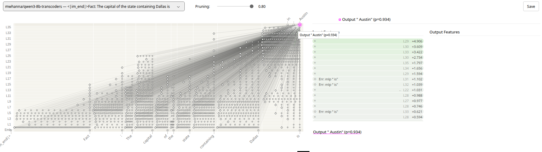
Switching those three Texas features off dropped Austin from 0.935 to 0.38, and
Atlanta rose to 0.34. That is a real causal effect. It is also one prompt that I
picked because the picture looked clean.
I spent fifteen years validating server CPUs. One passing test case is not coverage, and a debug theory that explains the failure you were staring at is the one most likely to be wrong in general. So I treated the graph's story as a hypothesis and wrote a test plan for it.
Turning the picture into a test suite
Fifty-seven city, state, capital triples, using well-known cities that are not capitals. I skipped state pairs whose names collide, such as the two Carolinas, and cities whose names contain a state. Every prompt uses the same template. The model answers 50 correctly; the seven misses (San Diego, Orlando, Rochester, Reno, Norfolk, Wilmington, Manchester) are excluded, and one more has no labelled features, which leaves 49.
For each prompt the suite:
- Builds the attribution graph and keeps the pruned nodes (80% of influence) at the city token and the final token, roughly 600 features per prompt.
- Labels state features with an oracle that never looks at the graph. A feature counts as a state feature if its own top output tokens, taken from the published feature data, name that state. Texas features predict Texas, Texans, Tex. This keeps the test from grading the graph against itself.
- Ablates the labelled state features, setting them to zero, and records the probability of the correct capital.
- Runs a control: zero the same number of randomly chosen non-state features from the same graph, at the same token positions, three draws per prompt. These are influential features too; they survived the same pruning.
- Swaps: zero the state features and inject another state's features from a donor prompt at their recorded activations, at 1× and 2× strength. If the claim is right, Dallas plus California features should say Sacramento.
The state features are causal
Switching off the state features drops the median probability of the correct capital from 0.97 to 0.18. In 31 of 49 prompts it falls below 0.5. The random control, with the same number of features from the same graph, leaves the median at 0.96 and never falls below 0.5.
Show data table
| City | Capital | Before | State off | Random off | Labelled features |
|---|---|---|---|---|---|
| Tampa | Tallahassee | 0.93 | 0.00 | 0.94 | 12 |
| Miami | Tallahassee | 0.96 | 0.00 | 0.90 | 10 |
| Philadelphia | Harrisburg | 0.92 | 0.00 | 0.91 | 8 |
| Louisville | Frankfort | 1.00 | 0.00 | 1.00 | 4 |
| Newark | Trenton | 1.00 | 0.00 | 1.00 | 4 |
| Worcester | Boston | 0.94 | 0.00 | 0.94 | 6 |
| Chicago | Springfield | 0.84 | 0.00 | 0.81 | 7 |
| San Antonio | Austin | 0.96 | 0.00 | 0.96 | 11 |
| Detroit | Lansing | 0.97 | 0.00 | 0.95 | 11 |
| Dallas | Austin | 0.94 | 0.00 | 0.88 | 13 |
| Houston | Austin | 0.99 | 0.00 | 0.99 | 11 |
| Knoxville | Nashville | 0.45 | 0.00 | 0.61 | 7 |
| Bangor | Augusta | 0.95 | 0.00 | 0.81 | 7 |
| Flagstaff | Phoenix | 0.98 | 0.01 | 0.86 | 7 |
| Billings | Helena | 0.91 | 0.01 | 0.90 | 5 |
| New Orleans | Baton Rouge | 0.94 | 0.01 | 0.51 | 11 |
| Tucson | Phoenix | 1.00 | 0.01 | 0.99 | 5 |
| Hilo | Honolulu | 0.87 | 0.02 | 0.86 | 14 |
| Huntsville | Montgomery | 0.92 | 0.03 | 0.92 | 7 |
| Wichita | Topeka | 1.00 | 0.07 | 1.00 | 11 |
| Memphis | Nashville | 0.96 | 0.08 | 0.97 | 5 |
| Boulder | Denver | 1.00 | 0.10 | 1.00 | 11 |
| Cedar Rapids | Des Moines | 0.94 | 0.12 | 0.91 | 7 |
| Pittsburgh | Harrisburg | 0.91 | 0.12 | 0.88 | 8 |
| Milwaukee | Madison | 0.99 | 0.18 | 1.00 | 8 |
| Fayetteville | Little Rock | 0.50 | 0.20 | 0.52 | 4 |
| Cincinnati | Columbus | 0.90 | 0.20 | 0.90 | 6 |
| Los Angeles | Sacramento | 1.00 | 0.21 | 0.99 | 18 |
| New Haven | Hartford | 0.97 | 0.22 | 0.94 | 6 |
| Savannah | Atlanta | 0.99 | 0.24 | 0.99 | 7 |
| Spokane | Olympia | 0.65 | 0.31 | 0.69 | 7 |
| St. Louis | Jefferson City | 0.92 | 0.59 | 0.95 | 4 |
| Sioux Falls | Pierre | 0.63 | 0.60 | 0.66 | 1 |
| San Francisco | Sacramento | 0.99 | 0.72 | 0.99 | 16 |
| Las Vegas | Carson City | 0.80 | 0.81 | 0.82 | 3 |
| Albuquerque | Santa Fe | 0.85 | 0.84 | 0.86 | 1 |
| Anchorage | Juneau | 1.00 | 0.85 | 1.00 | 7 |
| Eugene | Salem | 0.97 | 0.86 | 0.97 | 6 |
| Biloxi | Jackson | 0.96 | 0.87 | 0.96 | 3 |
| Provo | Salt Lake City | 0.99 | 0.88 | 0.99 | 9 |
| Omaha | Lincoln | 0.97 | 0.90 | 0.97 | 2 |
| Baltimore | Annapolis | 0.99 | 0.93 | 0.99 | 7 |
| Cleveland | Columbus | 0.97 | 0.99 | 0.96 | 5 |
| Bridgeport | Hartford | 0.99 | 0.99 | 1.00 | 7 |
| Charlotte | Raleigh | 0.99 | 0.99 | 0.99 | 3 |
| Casper | Cheyenne | 1.00 | 0.99 | 1.00 | 3 |
| Seattle | Olympia | 1.00 | 1.00 | 0.99 | 6 |
| Burlington | Montpelier | 1.00 | 1.00 | 1.00 | 3 |
| Mobile | Montgomery | 1.00 | 1.00 | 1.00 | 8 |
The failure mode is informative. In 11 of the collapsed prompts the model still names a state
capital, just the wrong one: Dallas, Houston and Miami all become Atlanta. The
request for a capital survives; only the knowledge of which state is gone. That is what you
would expect if "capital of" and "which state" are carried separately, which is the two-hop
story the graph told.
Freezing attention patterns during the intervention is the library default. Letting attention respond gives the same picture: 28 of 49 collapse, against 2 of 49 for the random control.
Swapping states mostly works, if you push
At the donor's recorded activation strength, swapping in another state's features makes the
model answer with the donor's capital in 15 of 49 prompts. At twice the strength it happens in
28 of 49. Dallas with California features says Sacramento. Detroit with Ohio
features says Columbus. Newark with Massachusetts features says Boston.
Swaps fail mostly when the donor state has few labelled features: a median of 5 for failed swaps at 2×, against 8 for successful ones. That points at the labeller's coverage again, which is the question the next section takes up.
The 18 that did not break
Eighteen prompts barely moved when their state features were switched off: Seattle, Charlotte, Burlington, Mobile and others. They have fewer labelled state features (a median of 4.5, against 7 for the prompts that collapsed). There are two explanations. Either the labeller is missing state features for these cities, or the model reaches the capital some other way, for example a direct association between Seattle and Olympia that never passes through "Washington", or a path that bypasses the transcoders through their error terms.
A blunt diagnostic separates part of that. Switching off every graph feature at the city
token, labelled or not, about 300 per prompt, breaks all 18. So the answer does flow through
transcoder features at the city token, not around them. The test is blunt because it also
erases the city itself; many answers degrade to in or located.
What it rules out is the bypass. What it does not settle is whether the features my labeller
missed encode the state or a direct city-to-capital link. That is the next experiment.
| City | Before | State off | All city off | City features |
|---|---|---|---|---|
| Mobile | 1.00 | 1.00 | 0.00 | 268 |
| Burlington | 1.00 | 1.00 | 0.00 | 407 |
| Seattle | 1.00 | 1.00 | 0.01 | 186 |
| Casper | 1.00 | 0.99 | 0.00 | 498 |
| Charlotte | 0.99 | 0.99 | 0.00 | 377 |
| Bridgeport | 0.99 | 0.99 | 0.00 | 455 |
| Cleveland | 0.97 | 0.99 | 0.00 | 299 |
| Baltimore | 0.99 | 0.93 | 0.06 | 244 |
| Omaha | 0.97 | 0.90 | 0.00 | 341 |
| Provo | 0.99 | 0.88 | 0.00 | 613 |
| Biloxi | 0.96 | 0.87 | 0.24 | 154 |
| Eugene | 0.97 | 0.86 | 0.00 | 400 |
| Anchorage | 1.00 | 0.85 | 0.01 | 294 |
| Albuquerque | 0.85 | 0.84 | 0.00 | 302 |
| Las Vegas | 0.80 | 0.81 | 0.00 | 292 |
| San Francisco | 0.99 | 0.72 | 0.01 | 224 |
| Sioux Falls | 0.63 | 0.60 | 0.00 | 380 |
| St. Louis | 0.92 | 0.59 | 0.00 | 338 |
What this is and isn't
It is one model, one relation and one prompt template, tested over two days. The labeller matches output tokens against state names, so it can miss features that encode a state without predicting its name, and ambiguous names such as Washington and Georgia can fool it. Candidates come only from the pruned graph at two token positions. Probabilities are measured on the first token of the capital. All of these are deliberate simplifications that the data files make easy to revisit.
What it shows is a way of working I trust: take a mechanistic claim, make the oracle independent of the tool that produced the claim, put a control next to every intervention, and report where the claim breaks as carefully as where it holds. The 18 holdouts are the most interesting rows in the table.
Source and raw data
Every number above comes from these files.
Code and data are also on GitHub: github.com/j-curreri/two-hop-circuit-validation.